HELP
SWiFT-Helio1D is an automated pipeline to predict ambient solar wind properties using one-dimensional solar wind propagation modelling. With the modeled solar wind emergence near the Sun, the SWiFT-Helio1D provides modeling of solar wind properties at 1AU, this includes stream interaction regions, which can cause geomagnetic disturbances including enhancements of energetic electron fluxes in the Earth’s radiation belts (potentially harmful to communication satellites), at L1 upstream of the Earth up to 4 days in advance.
Introduction
Stream interaction regions are formed when fast solar wind stream originated from the coronal holes overtake slow solar wind stream or as they propagate outward from the Sun. As these structures often corotate with the Sun, they are also called Corotating Interaction Regions (CIRs). CIRs are the main drivers of geomagnetic disturbances in an absence of Coronal Mass Ejections, in particular, during the declining phase and the solar minimum of a solar cycle. Communication satellites in the geostationary orbit and medium and low Earth orbits (i.e., GEO, MEO, and LEO, respectively) are in the vicinity of the Earth's radiation belts: the regions encircling the near-Earth space and containing significant fluxes of high-energy electrons and ions. The SWiFT-Helio1D pipeline can be used to provide solar wind conditions to drive existing magnetospheric and radiation belt models that encompass the GEO, MEO, and LEO. Since the beginning of space technology era, there have been a number of reports of spacecraft anomalies and even failures, for example, at the geostationary orbit due to the elevated fluxes of several MeV electrons that persisted for several days following CIRs (see a review by Lanzerotti, 2007). With the real-time monitoring of the solar wind at the Lagrangian L1 point, e.g. by Advanced Composition Explorer (ACE) satellite, the continuous prediction of the radiation belt conditions via modeling is limited to one hour in advance as the solar wind takes about 40 - 60 minutes from L1 to arrive at the magnetosphere.
To mitigate the impacts of space weather on telecommunication satellites, advancing the lead time of the prediction is a critical task. "Helio1D" has been developed under the STORMS-SWiFT framework to nowcast and forecast ambient solar wind conditions (speed, density, temperature, tangential magnetic field) at L1 with a lead time of 4 days. The Helio1D pipeline connects two models namely Multi-VP (Pinto & Rouillard, 2017) for modeling solar wind emergence and 1-D magnetohydrodynamics (MHD) (Tao et al., 2005) for modeling solar wind propagation and CIR formation. Both models have been developed and further extended at IRAP with an objective to provide operational space weather services at Earth and in the heliosphere (André et al. 2018; Rouillard et al. 2020). In the framework of the EU H2020 SafeSpace project (Daglis, 2022), for example, we have evaluated the forecasting of electron fluxes along the trajectory of one the Galileo satellites (GSAT215) with solar wind prediction from the SWiFT-Helio1D pipeline. Moreover, it can also potentially be used with other satellites upon evaluation when the electron flux data along the orbit of specific satellites are available (Dahmen et al. 2023).
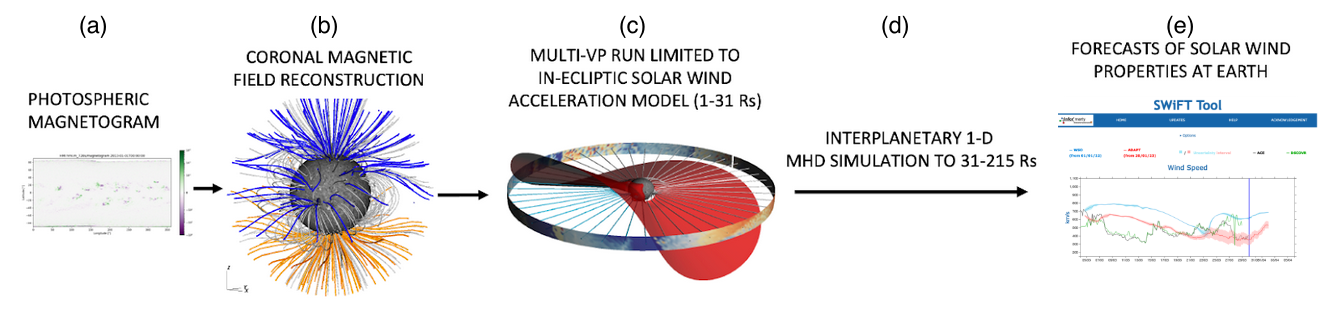
Figure 1 shows a schematic architecture of the SWIFT modelling framework. In Fig 1a, the daily synoptic map of photospheric magnetogram from ground observations is first processed. The processed magnetogram is then ingested to reconstruct the coronal magnetic field as shown in Fig 1b. At this step, the solar coronal field is reconstructed using an empirical approach (using the magnetostatic potential field source surface (PFSS) extrapolation). Next, the Multi-VP model (Pinto & Rouillard, 2017) computes the solar wind emergence, based on the reconstructed solar corona, that covers the heliocentric distances over which all solar wind streams are formed and accelerated between 1 and about 31 solar radii as shown in Fig 1c. Here, MULTI-VP determines a full set of physical quantities in 3-D consisting of solar wind speed (V), density (n), temperature (T), and magnetic field (B) in the equatorial plane (see more in “‘Brief methodology” below’). These solar wind properties, generated at the sub-Earth point at 0.14 AU (at 31 solar radii), are then ingested into the 1D MHD model as shown in Fig 1d. The 1D MHD model subsequently propagates the solar wind emergence at 31 solar radii to 215 solar radii (about 1 AU) while taking into account the interaction between the fast and slow solar wind streams radially away from the Sun. The SWiFT-Helio1D finally provides forecasts of solar wind properties at Earth as shown in Fig 1e.
Here, we provide daily ensemble nowcasting and forecasting of 21 solar wind time series, consisting of several targets around the Earth to account for the uncertainties, from day D-3 to D+4 for any given day D. Helio1D can be used to provide daily solar wind forecasting at L1 or feed real-time, daily solar wind forecasting to predict the dynamics of the inner magnetosphere and the radiation belts.
Brief methodology
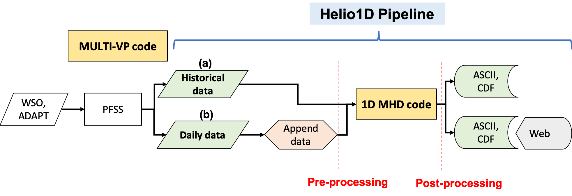
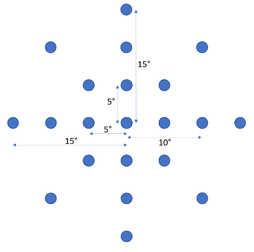
We developed an interface to automate the connection between the solar wind prediction near the Sun at 0.14 AU by Multi-VP and the propagation to 1 AU (at L1) by 1D MHD (see Figure 2). Using daily magnetograms from Wilcox Solar Observatory (WSO) and the flux transport model ADAPT (Air Force Data Assimilative Photospheric Flux Transport), Multi-VP is set to automatically generate daily solar wind forecasting at the sub-Earth point and the surrounding virtual targets up to 15o in latitude and longitude (see Figure 3) 2 days in advance. The spread of the virtual targets in addition due to the sub-Earth point as shown in Figure 3 is motivated from the fact that the magnitude of the solar wind speed profiles is different at different heliospheric latitudes as a function of the warping of the Heliospheric Current Sheet and nearby velocity gradients. Therefore, the modeling of solar wind profiles at the virtual targets can provide the timing and magnitude uncertainties. On SWiFT-Helio1d website, the errors are given as the standard deviation from the 21 one-dimensional solar wind solutions calculated for the virtual targets around the sub-Earth point, given by the Multi-VP model, shown in Figure 3. All the 21 solar wind time series are available to download (see “Data products” below).
Multi-VP determines a full set of physical quantities consisting of 3-D solar-wind velocity (V), density (n), temperature (T), and 3-D magnetic field (B). To propagate this solar wind emergence through the heliosphere using 1D MHD, we keep the tangential magnetic field component to physical values while the radial magnetic field is fixed to 0.001 nT to meet the solenoidal criterion, and the Bz is set to zero (see Tao et al., 2005 for discussion). By propagating this solar wind to Earth, we gain an extra lead time of 2 – 7 days depending on the solar wind speed; we limit this time to 2 days for a total lead time of 4 days from Helio-1D. Furthermore, the 1D MHD code requires a sufficiently long time-series to cover at least 1 solar rotation (27.5 days). We concatenate the daily Multi-VP time series together by averaging the data from D-30 to D for a given day D to make the time series inputs to be sufficiently long. In addition, some values of Multi-VP data may be unphysical (due to the poor quality of magneograms and/or numerical effects). We apply a set of criteria to correct those values. The concatenation process was set to prioritize (1) the dataset nearer to the day in which the model is run, (2) the dataset which has minimum number of unvalid values, and (3) the dataset which is the most contigous from the previous data (in order to limit discontinuities).
The coordinate system in the 1D MHD code is equivalent to the Radial-Tangential-Normal (RTN) system, where the X-axis (R) is pointing radially outward from the Sun in the equatorial plane to the Earth, the Z-axis (N) is the solar rotation axis, and the Y -axis (T) completes the orthonormal system. The outer boundary is set to 1.4 AU where the derivatives of all physical parameters diminish. The Helio1D outputs solar wind speed, number density, temperature, and tangential magnetic field (called BY). We note that the Helio1D cannot provide a physical Bz due to its limited dimensionality. In fact, even a 3D model would hardly give any physical BZ because BZ in CIRs is very variable primarily owing to large-scale Alfvén waves (e.g., Lavraud et al. 2010), which no model is currently able to reproduce. Nevertheless, we may infer that the maximum amplitude of BZ is the same as the absolute value of the tangential magnetic field because both BY and BZ are the components perpendicular to the main solar wind flow and will typically experience the same compression (through stream interactions) during propagation to 1 AU. In other words, the BZ value that is provided here may be used as an envelope (-BZ to + BZ) of the possible BZ value at 1 AU at all times. At the moment, we do out display BZ but instead show only the tangential magnetic field component BY. In addition, when the lead time of the time series output from Helio1D is shorter than 4 days, we fill the series using the latest available values to fit the required data length. Though this approach minimizes data gaps, it can lead to constant values in outputs.
Using historical data in 2005 – 2012 and 2017 – 2018, we benchmarked the quality of solar wind modeling from Helio1D against the observations at L1 using the OMNI dataset. We find that the metrics such as root-mean-square errors (RMSE) show relatively low values, around 80 km/s, during the solar minimum. The RMSE and similar metrics positively correlate to the number of sunspots (Kieokaew et al. 2023). Moreover, we find that the solar wind number density and temperature at the CIR are typically higher than those of the observations. This is due to the over-compression as the 1D MHD code is based on an ideal MHD plasma assumption (i.e., no dissipation) and a limited dimensionality. To correct for this numerical effect, we apply a linear function to lower the number density and temperature of the output. The Helio1D pipeline has been operational and available through the SWiFT platform since the 10th of January 2022.
Model uncertainties
The uncertainties of the model, shown as shaded area around the solid line in each plot, are computed from the standard deviation of all the 21 SWiFT-Helio1D solar wind solutions calculated for the virtual targets around the sub-Earth point (given by the Multi-VP model) as shown in Figure 3. These uncertainties include both timing and magnitude uncertainties as the different solar wind solutions at the various targets would predict different arrival times and magnitudes of stream interfaces. All the 21 solar wind solutions are available to download (see “Data products”) below.
Data products
SWiFT-Helio1D provides daily nowcasting and forecasting of the background solar wind conditions, covering from D-27 to D+3 for any given day D, given as 21 time series at the 1-hr cadence in UTC time. The solar wind conditions are provided for the bulk flow speed (V), number density (n), temperature (T), and one-dimensional magnetic field in the tangential direction (BT in the Radial-Tangential-Normal system, equivalent to -BY in the Geocentric-Solar-Ecliptic system).
Note that the time interval covers D-27 to D+7. Future enhancements on SWiFT-Helio1D will cover this whole interval.
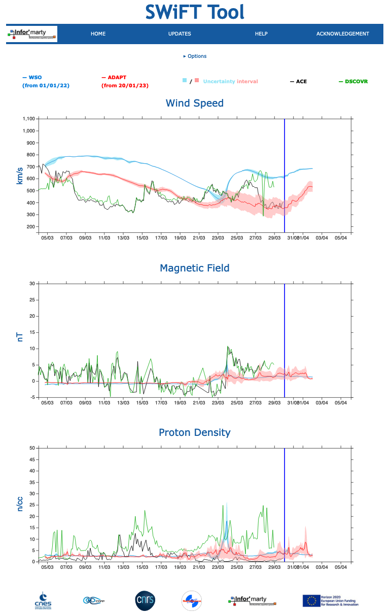
The data are generated in a self-describing Common Data Format (CDF) at about 6 am every day. The quick-look of data is available daily for the average and the standard deviation of all solar wind time series. An example is shown here in Figure 4.
The daily files are publicly available for download via the API:
WSO : https://swift-ssa-esa_irap_omp_eu.content.swe.s2p.esa.int/api/wso/YYYY-MM-DD/ (please indicate the date in YYYY-MM-DD format, e.g., 2022-03-01 for the 1st of March, 2022.)
ADAPT : https://swift-ssa-esa_irap_omp_eu.content.swe.s2p.esa.int/api/adapt/YYYY-MM-DD/ (No data before 20/01/23; same format for the date)
Caveats
Helio1D is sensitive to the quality of the input magnetograms that are used as the daily input (i.e., for constructing the inner boundary conditions) of Multi-VP. To date, we have used the daily WSO synoptic magnetograms as inputs as we have extensively benchmarked the pipeline using the longest historical data only available by WSO. Outputs using WSO are available from 10/01/2022 onwards. When the daily WSO magnetograms are unavailable, the Helio1D pipeline has been set to run using magnetograms of the previous solar rotation (using an assumption that the coronal structures are similar to the previous solar rotation and that we expect a consistent CIR formation to the previous rotation). We have recently added ADAPT magnetogram source (specifically ADAPT 1) to our pipeline. Helio1D outputs using ADAPT are available from 20/01/2023 onwards. Please note that we have not performed an exhaustive benchmarking of this magnetogram, and the data are not available for downloading. The outputs from ADAPT will be available for downloading upon the test of their performance.
Future development
An adaptation to change to another source of the daily magnetograms (e.g., GONG-ADAPT) is planned for Helio1D in 2023 upon validation. A more realistic inner boundary condition (e.g., initial radial magnetic field) and more inner heliospheric physics such as solar wind acceleration will be considered and integrated into the pipeline upon validation.
Acknowledgements
The work has received funding from the European Union’s Horizon 2020 research and innovation programme under grant agreement No 870437 for the SafeSpace (Radiation Belt Environmental Indicators for the Safety of Space Assets) project. Work at IRAP is also supported by the Centre national de la recherche scientifique (CNRS), Centre national d'études spatiales (CNES), and the University of Toulouse – Paul Sabatier (UPS).
References
- André, N., M. Grande, N. Achilleos, M. Barthélémy, M. Bouchemit, K. Benson, P. L. Blelly, et al. 2018. “Virtual Planetary Space Weather Services Offered by the Europlanet H2020 Research Infrastructure.” Planetary and Space Science 150 (April 2017): 50–59, doi:10.1016/j.pss.2017.04.020
- Daglis, I. A. and the SafeSpace Team: Advanced Prediction of the Outer Van Allen Belt Dynamics and a Prototype Service: the H2020 SafeSpace project , EGU General Assembly 2022, Vienna, Austria, 23–27 May 2022, EGU22-6518, doi:10.5194/egusphere-egu22-6518
- Dahmen, N., Brunet, A., Bourdarie, S., Katsavrias, C., Bernoux, G., Doulfis, S., Nasi, A., Papadimitriou, C., Oliveros Fernandez, J., and Daglis, I.: Electron radiation belt safety indices based on the SafeSpace modelling pipeline and dedicated to the internal charging risk, EGUsphere [preprint], doi:10.5194/egusphere-2022-1509, 2023
- Kieokaew, R., R. Pinto, M. Indurain et al. (2023), “Physics-based model of solar wind stream interaction regions: interfacing between Multi-VP and 1D MHD for operational forecasting at L1”, submitted to Journal of Space Weather and Space Climate. http://arxiv.org/abs/2303.09221
- Lavraud, B, A Opitz, J. T. Gosling, A. P. Rouillard, K Meziane, J. A. Sauvaud, A Fedorov, et al. 2010. “Statistics of Counter-Streaming Solar Wind Suprathermal Electrons at Solar Minimum: STEREO Observations.” Annales Geophysicae 28 (1): 233–46, doi:10.5194/angeo-28-233-2010.
- Lanzerotti, L. J. (2007). Space weather effects on communications. In V. Bothmer & I. A. Daglis (Eds.), Space Weather- Physics and Effects (p. 247), doi:10.1007/978-3-540-34578-7_9
- Pinto, Rui F., and Alexis P. Rouillard. 2017. “A Multiple Flux-Tube Solar Wind Model.” The Astrophysical Journal 838 (2): 89, doi:10.3847/1538-4357/aa6398
- Rouillard, A. P., R. F. Pinto, A Vourlidas, A De Groof, W. T. Thompson, A Bemporad, S Dolei, et al. 2020. “Models and Data Analysis Tools for the Solar Orbiter Mission.” Astronomy & Astrophysics 642 (October): A2, doi:10.1051/0004-6361/201935305
- Tao, Chihiro, Ryuho Kataoka, Hiroshi Fukunishi, Yukihiro Takahashi, and Takaaki Yokoyama. 2005. “Magnetic Field Variations in the Jovian Magnetotail Induced by Solar Wind Dynamic Pressure Enhancements.” Journal of Geophysical Research 110 (A11): A11208, doi:10.1029/2004JA010959